Note:
Over the past few months I've had an interesting, ongoing discussion with Allen Dominek regarding measuring chamber pressure using strain gauges. He has produced an excellent, and very technical article with the results of his work and has kindly allowed me to publish his article here.  Enjoy.

Roy Seifert
The Kitchen Table Gunsmith

Introduction
The measurement of gun's chamber pressure may provide useful diagnostic information for load design and barrel performance. There are three measurement techniques involved in chamber pressure measurements [1,2]. Historically, the standard was a CUP measurement which captured a peak chamber pressure using a compressible copper pellet. A more recent technique using a piezo sensor yields a more accurate measurement of not only peak pressure but of the pressure in the barrel as the bullet is accelerated. Both of these methods involve the modification of the gun to install the sensor. The third technique uses a strain gage which is placed over the chamber where the round is or at some other location along the barrel. Hence, such a measurement technique is non-invasive but not as accurate as the piezo sensor technique. A strain gage is a small electrical resistor which is sensitive to small compressive or expansive forces that the supporting surface experiences. A potential accuracy limitation does exist from the analytical formulas used to relate chamber pressure to strain and the placement of the sensor on the barrel.

Strain gages have been used for many years to measure deformations. One early study is found here [3]. A commercially available strain sensor system is available from Recreational Software, Inc. (RSI) [4]. Additional information on sensor preparation and measurement technique is available at [5].

The numerical data for the chamber pressure as a function of time permits additional diagnostic capability. One example is shown in [6]. Unfortunately, their mathematical derivation for a closed formula expression relating terminal barrel velocity and pressure is in error since it assumes a bullet velocity that is increasing linearly as a function of time. It is this work that made me interested in chamber pressure measurements using strain gages.

The following material outlines my activities for chamber pressure measurements and numerical processing. The activities include designing/building the pressure measurement hardware and numerically processing the measured data.

Pressure Measurement Hardware
When a round is fired in a chamber, a complex chemical process (powder burning) occurs to rapidly build up pressure to accelerate the bullet. This pressure can be measured using a strain gage attached to the exterior surface of the chamber since the chamber approximates an open pressure vessel. There are expressions relating the interior pressure of a vessel to the expansion of the vessel. The rifle chamber geometry is not exactly a traditional pressure vessel but these expressions can be used to estimate the chamber pressure.

The key to measuring this pressure is to be able to measure the strain that the internal pressure exerts upon the barrel. A strain gage provides an excellent sensor to do this. A strain gage is an electrical resistor which changes its resistance due to minute physical geometry changes [7,4,5].

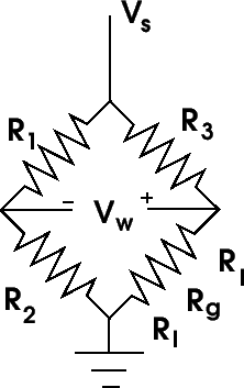
The measurement of this electric change requires the use of a Wheatstone bridge. There are a number of different Wheatstone bridge configurations available [8]. Figure 1 illustrates the typical resistive network. It consists of three additional resistors with the strain gage.

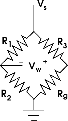
Figure 1: Basic Wheatstone bridge.

When R₁/R₂ = R₃/R_g the resistance of the sensor changes and this voltage is no longer zero since the bridge is no longer balanced. It is this voltage that is measured to obtain the pressure inside the chamber. The expression which relates voltage to strain is given in Equation 1 ([8])

where is the strain, is the normalized measured Wheatstone bridge voltage V_w/V_s with all the resistors equal R₁=R₂=R₃=R and R_g=R+∆R. The factor GF is the gage factor which has a value of around 2. This value is provided by the gage manufacturer and is the calibration factor for the gage relating the normalized resistance change to the strain. The gage factor is defined as

where ∆R is the resistance change of the strain gage.

Equation 1 was derived by expressing the differential voltage as

then setting R₁=R₂=R₃=R and solving for using the GF relationship in Equation 2.

When the Wheatstone bridge is physically realized, the sensor is typically physically removed from the other resistors and the impact of having connecting wires should be addressed. Figure 2 illustrates the electrical model.

Figure 2: Wheatstone bridge with sensor wire loss included.

The effect that the wires present is an additional loss component. This loss is very small but so is resistance change of the sensor. Equation 1 can be modified to account for this resistance and is

However, there is probably no reason to use this approximation with today's numerical calculation resources. It does demonstrate that the strain is primarily given by the first term and that the contribution of loss from the connecting wires to the strain gage is essentially a constant DC term which is about 100 times smaller than the first term for the given loss values.

There is a three wire sensor configuration [8] where a second wire is attached to one of the sensor pads. This is only effective for eliminating the loss in one of the wires so I find it not helpful and not really of value considering the size of R_l in my application.

Pressure/Strain Formulas
The next step is to relate the measured strain values to the internal pressure of a chamber. Approximate expressions can be found in [9]. The author attempted to relate the internal chamber pressure to the external strain on the barrel using expressions for thick and thin walled pressure vessels. The presentation was technically weak and resulted in the use of equations not appropriate for this application. These equations, however, did provide numerical values that were realistic in magnitude. A formulation to calculate the internal pressure of a chamber using measured strain data is presented below. It is a simple model and appears to be reasonable from the experimental testing presented later.

Traditional cylindrical pressure vessels are called "open" or "closed" A person may be tempted to classify a barrel as a "closed pressure vessel" but it is not. A closed pressure vessel has axial stresses induced by the internal pressures of the cylinder since the ends of the cylinder are physically constrained not to move. Also the classical "closed pressure vessel" has a steady state pressure throughout the cylindrical structure.

A rifle barrel is not a closed pressure vessel in the classical sense. Both ends are not mechanically constrained. The muzzle end is free to move. Placing a strain gage axially along the barrel will not sense any significant axial deformation when the round is fired. This means that the barrel can be modeled as an "open pressure vessel". Additionally, the pressure that the barrel is exposed to is transient in nature and not steady state (the entire barrel is not under a uniform pressure). The pressure wave, generated by firing the round, propagates down the barrel and does not sense the finiteness of the barrel until the pressure wave is at the muzzle. Until then, the barrel appears to be infinitely long. However, when the pressure wave does reach the muzzle, then additional interaction occurs. FEM modeling [10] confirms this simplistic model for early time.

There are a set of equations called Lame equations [11] describing the stresses in a cylindrical structure when the internal and external surfaces are under pressure. These stresses can be grouped into three types: circumferential, axial and radial. The only stress that is generated or is of significance when a round is fired in a gun is the circumferential stress.

The circumferential stress equation of interest is:

where p_i and p_o are the internal and external cylinder pressures, u=r_o/r_i is the ratio of the outer and inner cylinder diameters and r is a position between r_i and r_o. This equation is appropriate for what is termed "thick wall" where the cylinder radii are explicitly used.

Equation 6 can be specialized for two geometries, one for the barrel and one for the casing. In this model, the casing is in contact with the barrel's inner diameter. Such a geometry is typically called "compound cylinders". For the barrel, Equation 6 yields

and

where U_s is the ratio of the outer and inner diameters of the barrel where the strain gage is located and P_c is the contact pressure between the ID of the barrel and the outer diameter of the casing. Equation 9 is the pertinent equation for the casing:

where P_i is the internal pressure in the casing (barrel) and U_b is the ratio of the outer and inner diameters of the casing. Note that the subscript "s" refers to "steel" which is what the barrel is made from and the subscript "b" refers to "brass" which is what the cartridge is made from.

The desired equation to predict the interior pressure in a barrel by the measured strain on the exterior of a barrel is derived in two steps. The first step is to relate the change of circumference at the contact interface between the barrel and casing when a round is fired. Since both the barrel and casing are in contact during firing, both have to expand the same amount. This expansion is governed by the strain at the interface and has to be continuous at the contact boundary which requires:

The strain and stress of a material are related through a constant call Young's modulus or the modulus of elasticity, $E$ and is expressed as: 

Using Equations 8 and 9 with Equations 10 and 11 yields:

where the Young's modulus for steel (E_s), brass (E_b) and LDPE (shotgun shells) are 30*10^6, 16*10^6 and $0.13*10^6 psi, respectively. The contact pressure is determined by the strain gage reading. Using Equations 7 and 11 yields this contact pressure which is

Inserting P_c from Equation 13 into Equation 12 and reducing yields:

The accuracy in determining the chamber pressure is dependent upon many factors. From Equations 4 and 14, the factors are the measured Wheatstone bridge voltage (dependencies of strain gage bonding/orientation, the gage factor and amplifier gain), measured chamber/casing dimensions and the Young's modulus material constants. The only factors in which there are known uncertainties are the strain gage bonding quality to the barrel and the Young's modulus values.

The dimensions used in Equation 14 should be the dimensions under pressure. Fortunately for the amount of strain on the barrel, the change of the barrel dimensions under pressure is negligible. However, this is not the case for the casing. The outer diameter for the casing should be the inner diameter of the chamber since the case is in contact with the barrel during firing. This results in a thinner case thickness during firing than the case has under static conditions. The case thickness used in Equation 14 is scaled from the unfired case thickness. This scaling is based upon the fact that the amount of brass is constant. The thickness used is given by t₂=r₁t₁/r₂ where the subscripts refer to the dimensions before firing and 2 refer to the dimensions during firing. The change is negligible since the casing diameter expands roughly 0.004''.

Differential Amplifier Circuit
Modern operational amplifier (opamp) capabilities allow for very simple circuits to be made with superior electrical performance. Figure 3 illustrates one circuit that can measure the differential voltage generated by a Wheatstone bridge. A Texas Instruments INA129 instrumentation opamp is a device used to measure and amplify the generated differential voltage created by the sensor and reject the common mode voltage of the balanced bridge. The INA129 has the capability to have an adjustable gain through the resistance of R₅/R₆. This is important since different chambers and loads will have different pressure maximums. The gain is defined by 1+49.4k/R where R is either R₅ or R₆. A gain of 101 is provided when R₆ is 500 ohms and a gain of 26 is provide when R₅ is 2k. Of course, the actual gain should be measured to obtain the most accurate value for the gain.

The required gain can be estimated by calculating the expected pressures and voltages for various guns. The values shown in Table 1 for a 22LR rifle, a 12 gauge shotgun and a 7mm Mauser rifle are derived using Equations 12 and 13:

Calculated Wheatstone Voltages

Each gun requires a different amplifier gain if the maximum measured voltage is to be the same. The amplifier gains for the 22LR rifle, 12 gauge shotgun and 7mm rifle are 7100, 2300 and 1300, respectively, if the maximum measured voltage is 2.5 volts. The current instrumentation opamp has a gain limit of 10,000 but it is not good practice to use just one amplifier to achieve large gains. Another stage should be added. A fixed gain of 100 has been chosen for the second stage and it will have a low pass filter to attenuate higher frequency noise. The remaining gain will be provided by the first stage. A jumper has been provided to choose between two different gains of 25 and 100. These gains were chosen before the values in Table 1 were confirmed. A more appropriate set of gains would be 70, 22 and 12 or less.

All the components operate on a 5 volt rail supplied by a 9 volt battery (for portability) and a linear voltage regulator ADM7150. Opamp REF5020 provides an offset voltage for the instrumentation opamp output. Since the generated Wheatstone bridge voltage will be positive (as configured), it is necessary to offset the opamp output by a small voltage when the bridge is balanced. This is achieved by offsetting the INA129 output voltage by 2 volts using REF5020. The gain and offset voltage should be set so that the maximum output voltage is less than 4.5 volts for maximum sensitivity.

The other opamp, an OPA320, provides the remaining gain. The gain bandwidth product for this opamp is low so when a gain of 100 is used, the gain naturally rolls off to minimize the noise at the higher frequencies from being significant. The roll off starts around 4-5 kHz which is the upper frequency content limit of the signal of interest to be measured. From numerical modeling, slightly better noise performance is achieved when an OPA333 is used instead of an OPA320.

The circuit uses another multi-turn potentiometer, R3, to balance the bridge when the sensor has no strain on it. This adjustment is made to have pin 6 the same voltage as pin 5 on the INA129 opamp when the strain gage is in its nominal state. I make the adjustment so that the output voltage of the second stage is the same voltage the reference voltage provided by REF5020. If this is not done, the amplified voltage may be railed (at 5 volts) since the gain of the circuit is quite large.

A number of connection points (H1, H2, H3 and PH1) are present. PH1 provides for the connection of the 9v battery. H1 is the connection point for the strain sensor. H3 is a measurement point for both the pre-filtered (pin 1) and filtered (pin 3) amplified voltage. Jumper H2 permits for two discrete gain values to be chosen for the INA129 amplifier allowing maximum sensitivity depending upon the peak chamber pressure.

Note that the measured voltage value used in Equation 1 has to be divided by the total gain of the opamp circuit to recover the Wheatstone bridge voltage.

Numerical Processing
The velocity of the bullet and its position in the barrel can be estimated once the pressure in the chamber has been acquired. Note that the following derivation is under ideal conditions which are not met in a real life gun chamber/barrel. The calculated quantities are based upon many assumptions. As previously mentioned, the measurement and resulting pressure values have limitations. In this section, no account of all the energy created by the powder is attempted. Losses include heating, friction and bullet dynamics.

The force acting on a bullet is the gas expansion created by the burning of the powder. Considering Newton's Second Law of Motion as was done in [6], the bullet's motion can be roughly modeled by equating its mass and acceleration to the chamber pressure over its cross sectional area as

where m is the mass of the bullet, a is the acceleration, P is the chamber pressure and A is the area of the bullet. Expanding the a as the second time derivative of position yields:  

since

Realizing that:

results in Equation 16 becoming:

Multiplying both sides with dt and integrating yields:

where v1 and v2 are the velocities of the bullet at times t1 and t2, respectively. The integration approach used in [6] is basically wrong. I feel that there is no value in defining an average pressure as was done and the velocity of the bullet is not linear so one cannot say that

What can be determined by using Equation 20 is the velocity and position as a function of time by piece-wise integrating this equation. This is readily achieved since the measured data would be sampled with small, uniform temporal spacings. The velocity is determined by this equation:

where ∆t=t_i-t_i-1 and the position is determine by this equation:

The initial values for velocity and position are both zero. The final velocity is the muzzle velocity of when the bullet exits the barrel and the final position is the length of the barrel starting from the location of the bullet before it was fired.

There is one last consideration to make before calculating velocities and travel distances which is the resistance the bullet experiences traveling through the barrel. There are two types of resistance to account for. One resistance is the friction occurring between the bullet and the barrel and the classical friction model is speed independent. The other resistance is provided by the column of air that has to be quickly displaced as the bullet is going through the barrel. This resistance will be grouped into the friction resistance since no measurements were made to isolate this resistance.

For friction, there is a static and a kinetic friction. The static friction is a friction that is over come by the application of certain force (pressure*area). Once the bullet has started to move, there is a kinetic friction which is less than the static friction. These frictions impacts the calculation of the velocity and travel distance. These parameters (velocity and distance) can not be calculated until the chamber pressure achieves a certain level. At this level the bullet moves from the casing and is forced into the barrel where the rifling ID is smaller than the bullet diameter. At this point, kinetic friction is important. Part of the force on the bullet created by the chamber pressure is used to overcome this kinetic resistance. This remaining pressure is used for the velocity and distance calculations.

Data Collection
The pressure, velocity and distance equations presented in the previous sections are used with measured data. The first set of data was acquired from the internet at [10]. The provided pressure curves were manually digitized. Three other examples are presented that were acquired through the circuit described above. The examples are for a Remington Model 510 22LR rifle, a 12 gauge shotgun and a 7x57 mm Mauser rifle.

A Tektronix MDO3104 oscilloscope was used to measure and digitally collect the amplified Wheatstone voltages. The measured voltages were AC coupled to remove the DC offsets in the measurements. There are two sources for the DC offsets. One is from the offset generated by the REF5020 to shift the signal from 0 volts (since the opamps were single ended). The other offset is from the contribution of the finite lead resistance shown in Equation 5. The alternate approach to account for these offset would be to measure the DC voltage levels before the cartridge is fired and subtract this level from the time varying voltage measurements.

The physical circuit used in the measurements is shown in Figure 4. A nine volt battery was used to supply power to the circuit. The wires to the right provided measurement points for the first and second stage amplifiers. The two position terminal block on the top was were the strain gage wire were attached.

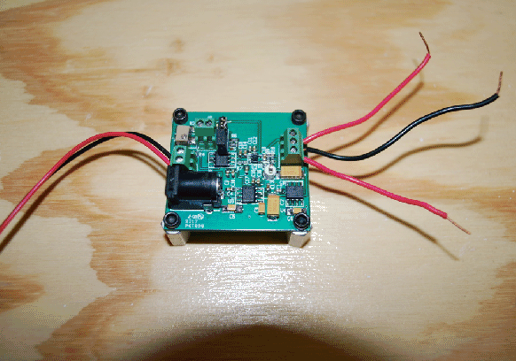
Figure 4: The physical pcb used in the measurements.

The static and kinetic friction forces were found using a numerical downhill simplex optimizer. The optimizer found the effective forces (pressures) which the calculated velocities and distances matched measured values. The measured velocities were provided by the ammunition manufactures and the distances from the measured barrel distances. The functional optimized was:

The pseudo code illustrating how the effective friction forces were determined is

  if(pres\_meas > fric\_static) then

      pres\_meas = pres\_meas - fric\_kinetic

      continue to determine velocity and distance 

  end if

where pres_meas is the chamber pressure found in Equation 14 and the friction values are determined through the downhill simplex optimizer using the muzzle velocity and the distance the bullet traveled in the barrel. The friction forces are then calculated from the psi friction values by multiplying them with the cross sectional barrel area.

Table 2 contains the various parameters that were used in the calculations. The provided grain weight values were converted to slugs for the calculations using a factor of 1\7000.*32.174=4.44*10^-6.

Physical Parameters used for the Numerical Calculations

Internet Data
Measured pressure values for a 22LR rifle using a 40 grain, .224 caliber bullet in a 24.75'' long barrel can be found at [10] for two loads. Figure 5 illustrates measured chamber pressure values using RSI hardware and software for one of the loads. The reference indicates that the pressure curve has been calibrated but there is not sufficient information on how it was achieved.

Figure 5 : Measured pressure curve of a 22LR. The barrel pressure dropped to zero at the end of the traces.

The calculated velocity and position calculations using this pressure curve are shown in Figures 6 and 7. Table 3 contains the resulting data.

Generated Data for a 22LR

Figure 6: Calculated bullet velocity in the 22LR barrel. Red: no friction included; Green: friction included.

Figure 7: Calculated bullet position in the 22LR barrel. Red: no friction included; Green: friction included.

Remington Model 510 22LR Rifle

Measurements for a 22LR were performed and Figure 8 illustrates the mounted strain gage.

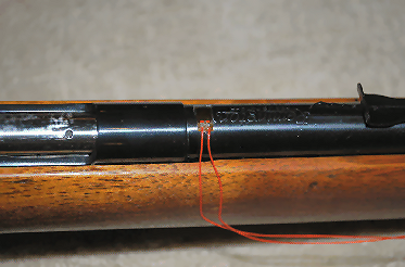
Figure 8: Strain gage illustration for the Remington Model 510 22LR rifle.

The chamber pressures are shown in Figure 9 based upon a circuit gain of 9880. The maximum measured voltage was 1.74 v which makes the maximum Wheatstone bridge voltage .17 mv. The receiver prevented the strain gage to be mounted over the casing of the round. Hence, no peak chamber pressures could be acquired. Note that there is a small pressure pulse before the main pulse around t=.5 ms. All the 2LR measurements had this behavior.

Figure 9 :Chamber pressure for the Remington Model 510 22LR rifle.

12 Gauge Shotgun
The mounted strain gage for a 12 gauge shotgun is illustrated in Figure 10. The shell used was 2.75'' with a shot weight of 1.125 ounces, Winchester AA light target load. The measured shot velocity using a chronograph was 1145 fps which is also the manufacture's reported shot velocity.

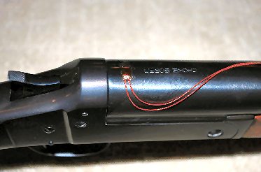
Figure 10: Strain gage illustration for a 12 gauge shotgun.

The chamber pressure is shown in Figure 11 based upon a circuit gain of 2470. The calculated velocity and position calculations using this pressure curve are shown in Figures 12 and 13. Table 4 contains the resulting data.

Figure 11: Chamber pressure for the 12 gauge shotgun.

Generated Data for a 12 Gauge Shotgun

Figure 12: Calculated shot velocity in the shotgun barrel. Red: no friction included; Green: friction included.

Figure 13: Calculated shot position in the shotgun barrel. Red: no friction included; Green: friction included.

7x57 mm Mauser Rifle
The mounted strain gauge for a 7x57 mm Mauser is illustrated in Figure 14. A Federal SP round was used with a reported muzzle velocity of 2660 fps.

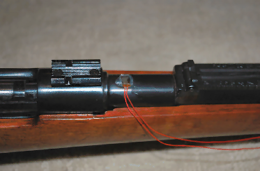
Figure 14: Strain gage illustration for the 7x57 Mauser rifle.

The chamber pressure is illustrated in Figure 15 with a circuit gain of 24.7. The red curve is measured data taken from the output of the first stage since the gain of the second stage was too large for this measurement. The green curve is post-processed data using a moving average. Note the pressure spike around .5 ms. This is when the bullet left the barrel.

Figure 15: Chamber pressure for the 7x57 Mauser. Note the pressure spike around .5 ms when the bullet left the barrel. The green curve is smoothed data using the data in the red curve.

The calculated velocity and position calculations using this pressure curve are shown in Figures 16 and 17. Table 5 contains the resulting data. Comparable results are obtained using either the raw or smoothed data from Figure 15.

Generated Data for a 7x57mm Mauser

Figure 16: Calculated bullet velocity in the Mauser barrel. Red: no friction included; Green: friction included.

Figure 17: Calculated bullet position in the Mauser barrel. Red: no friction included; Green: friction included.

Conclusions
The expressions derived and given here attempt to provide the chamber pressure from an analytical approach. It is seen that friction is an important factor in internal ballistics. This measurement approach can provide data on the static and kinetic friction for bullet/barrel interactions.

It was also observed that a better Wheatstone bridge nulling circuit, gain selection and amplifier configuration would be useful. Nulling the Wheatstone bridge to an absolute null is not critical as long as it is not too large to saturate the high gain amplifier. The residual offset voltage can be subtracted from the measurement or it can be blocked as was done in these measurements with the oscilloscope set to an AC input.

Figure 18 illustrates a possible nulling circuit. The nulling circuit now includes two trimmers instead of one. These trimmers provide a coarse and fine adjustment. This adjustment could be made automatic if a processor was used in conjunction with digital potentiometers.

Figure 18: Enhanced nulling circuit for the Wheatstone measurement circuit.

The amplifier configuration could also be changed to separate the amplification from the low pass filtering. The low pass filtering lessens the appearance of rapid pressure changes and rapid pressure changes potentially could be missed as was shown in the Mauser data. The current second amplifier stage could have its low pass filtering feature removed and a third stage added to provide low pass filtering with zero gain. If a third stage is not added for noise reduction, post processing with a moving average also could be used to remove the high frequency noise.

The observed chamber pressure characteristics were as anticipated except for the chamber pressure not going to zero once the bullet exited the barrel. This is bothersome but could be attributed to the thermal heating of the barrel and strain gage. A second strain gage could have been attached on the barrel to replace the fixed resistor, R1, in the Wheatstone bridge. This might have allowed a better, more natural balance in the nulling circuit. Another possibility for this behavior might be that the strain gage was not properly attached to the barrels. A Loctite 401 adhesive was used.

All the measured and calculated results depend upon the accuracy of the obtained pressure values. Any measurement has accuracy concerns. There are many measured parameters in this effort. The parameters are the physical dimensional measurements of the barrel and casing, the voltage measurements and the material properties of Young's modulus. Another accuracy consideration is that the numerical model using a simple compound cylinder to approximate a physical geometry (gun) may have its limitations.

Bibliography

1. Chamber Pressure, https://en.wikipedia.org/wiki/Chamber_pressure
2. Metallic Cartridge Chamber Pressure Measurement, http://www.chuckhawks.com/pressure_measurement.htm
3. Brownell, L.E., York, M., Sinderman, R., Jacob, K., Robbins H., "Absolute Chamber Pressure In Center-Fire Rifles", The University of Michigan, Industry Program of the College of Engineering, June, 1965, IP-710, https://deepblue.lib.umich.edu/bitstream/handle/2027.42/3866/
   bac6873.0001.001.pdf? sequence=5
4. Recreational Software, Inc., https://www.shootingsoftware.com/pressure.htm
5. Strain Gauges for Chamber Pressure Measurements, http:www.ktgunsmith.com /straingauge.htm
6. Calculating Barrel Pressure and Projectile Velocity in Gun Systems, http://closefocusresearch.com/calculating-barrel-pressure-and-projectile-velocity-gun-systems
7. Strain Gauge, https://en.wikipedia.org/wiki/Strain_gaug
8. Quarter Bridge, Half Bridge and Full Wheatstone Bridge Strain Gauge Load Cell Configurations, Transducer Techniques, https://www.transducertechniques.com/wheatstone-bridge.aspx
9. Strain Formulas, http://www.mindspring.com/$\sim$sfaber1/strnform3.htm
10. 22LR Rifle and Tuner, http://www.varmintal.com/a22lr.htm
11. Thick wall stress formulas. http://www.engineeringtoolbox.com/stress-thick-walled-tube-d_949.html